Julianna Renzi: Working with rasters

Read in the data

Read in some raster data on California cetaceans, which I’ll use in this example. These data are taken from AquaMaps (Kaschner, K., Rius-Barile, J., Kesner-Reyes, K., Garilao, C., Kullander, S., Rees, T., & Froese, R. (2016). AquaMaps: Predicted range maps for aquatic species. www.aquamaps.org). The data cover 35 Californian cetacean species and the probability of seeing each species at a given location given environmental factors such as depth, temperature, salinity, and proximity to shore. To see the code I used in each section click on the Show code option.

Show code

# get the names of rasters for each species
cet_tifs <- list.files(path = here("_posts", "2021-02-24-workingwithrasters", "ca_cetaceans"), pattern = ".tif", full.names = TRUE)

# bring rasters in as a raster stack
cet_stack <- raster::stack(cet_tifs)

# can view the object to make sure it looks correct:
cet_stack # looks good

class      : RasterStack 
dimensions : 12, 20, 240, 35  (nrow, ncol, ncell, nlayers)
resolution : 0.5, 0.5  (x, y)
extent     : -125, -115, 32, 38  (xmin, xmax, ymin, ymax)
crs        : +proj=longlat +datum=WGS84 +no_defs 
names      : Balaenoptera_acutorostrata, Balaenoptera_borealis, Balaenoptera_brydei, Balaenoptera_edeni, Balaenoptera_musculus, Balaenoptera_physalus, Berardius_bairdii, Delphinus_capensis, Delphinus_delphis, Eschrichtius_robustus, Eubalaena_japonica, Globicephala_macrorhynchus, Grampus_griseus, Indopacetus_pacificus, Kogia_breviceps, ... 
min values :                       0.11,                  0.02,                0.03,               0.03,                  0.01,                  0.06,              0.01,               0.03,              0.03,                  0.11,               0.59,                       0.02,            0.03,                  0.01,            0.03, ... 
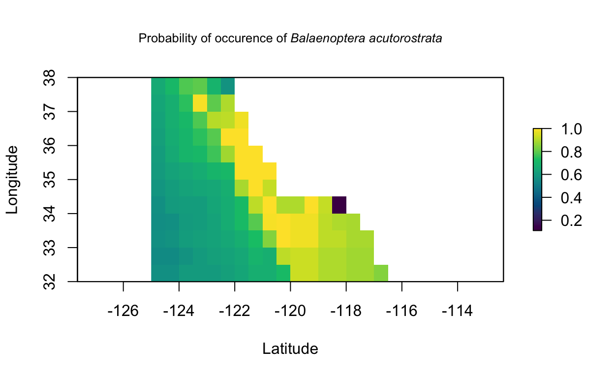
max values :                       1.00,                  1.00,                1.00,               1.00,                  1.00,                  1.00,              1.00,               0.63,              1.00,                  1.00,               1.00,                       1.00,            1.00,                  0.47,            1.00, ...

Plot the predicted distribution of a few species to examine the data. First for Balaenoptera acutorostrata:

Show code

plot(cet_stack$Balaenoptera_acutorostrata, col = hcl.colors(n = 100))
title(expression(paste("Probability of occurence of ", italic("Balaenoptera acutorostrata"))), cex.main = 0.8,
      xlab = "Latitude", ylab = "Longitude")

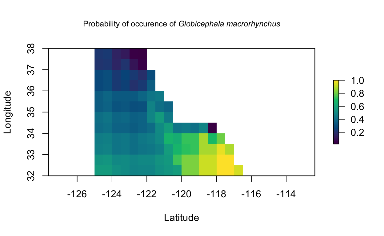
Then for Globicephala macrorhynchus:

Show code

plot(cet_stack$Globicephala_macrorhynchus, col = hcl.colors(n = 100))
title(expression(paste("Probability of occurence of ", italic("Globicephala macrorhynchus"))), cex.main = 0.8,
      xlab = "Latitude", ylab = "Longitude")

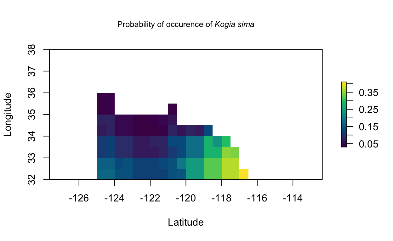
Then for Kogia sima

Show code

plot(cet_stack$Kogia_sima, col = hcl.colors(n = 100))
title(expression(paste("Probability of occurence of ", italic("Kogia sima"))), cex.main = 0.8,
      xlab = "Latitude", ylab = "Longitude")

Turn the data into presence/absence using raster algebra

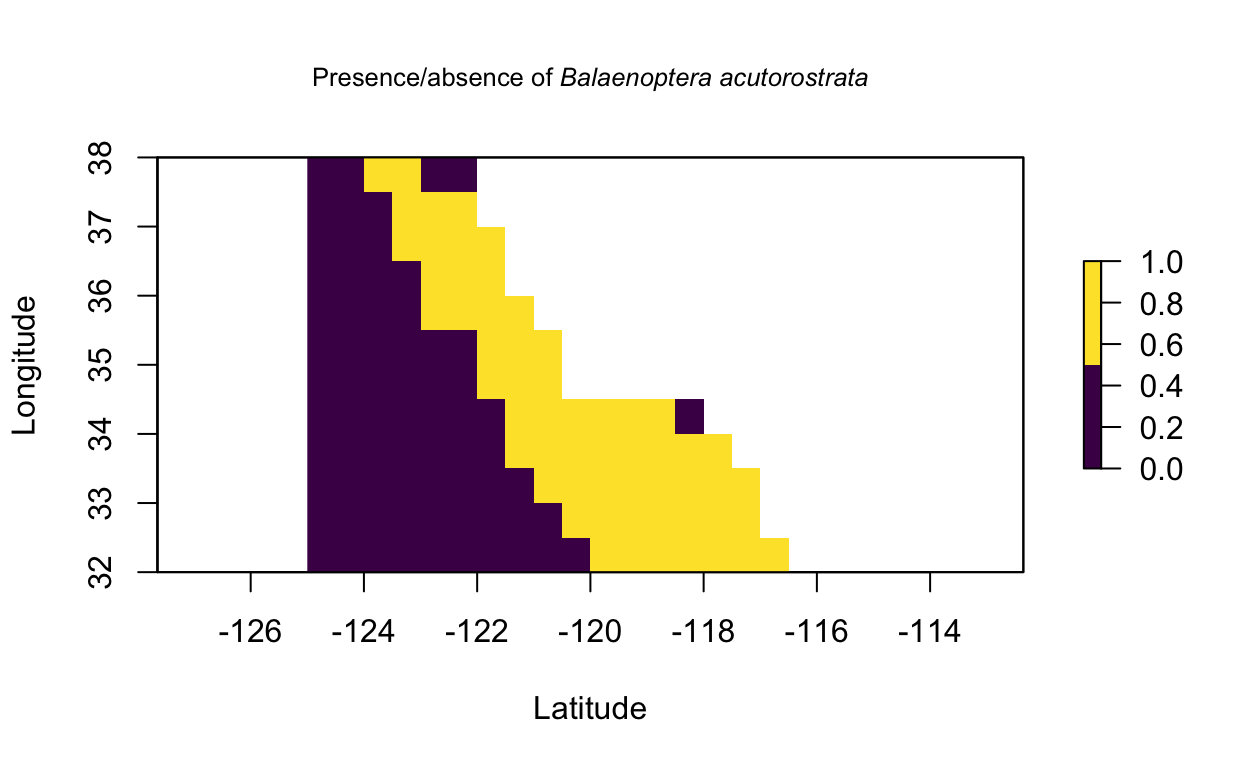
For the purposes of this exercise, we’ll define a species as likely to be “present” when the probability of observing it is greater than 0.75.

Show code

convert_pa <- function(x) {
  ifelse(x > 0.75, 1, 0)
}

cet_presence <- calc(cet_stack, function(x){convert_pa(x)})

Then we want to compare these plots with the modeled data above to make sure our function worked the way we wanted it to.

Here’s the output for Balaenoptera acutorostrata:

Show code

plot(cet_presence$Balaenoptera_acutorostrata, col = hcl.colors(n = 2))
title(expression(paste("Presence/absence of ", italic("Balaenoptera acutorostrata"))), cex.main = 0.8,
      xlab = "Latitude", ylab = "Longitude")

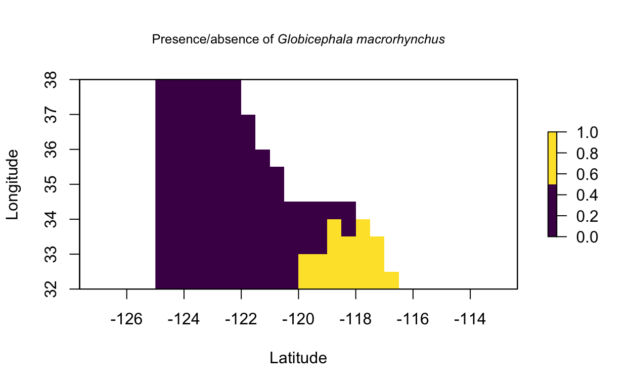
And for Globicephala macrorhynchus

Show code

plot(cet_presence$Globicephala_macrorhynchus, col = hcl.colors(n = 2))
title(expression(paste("Presence/absence of ", italic("Globicephala macrorhynchus"))), cex.main = 0.8,
      xlab = "Latitude", ylab = "Longitude")

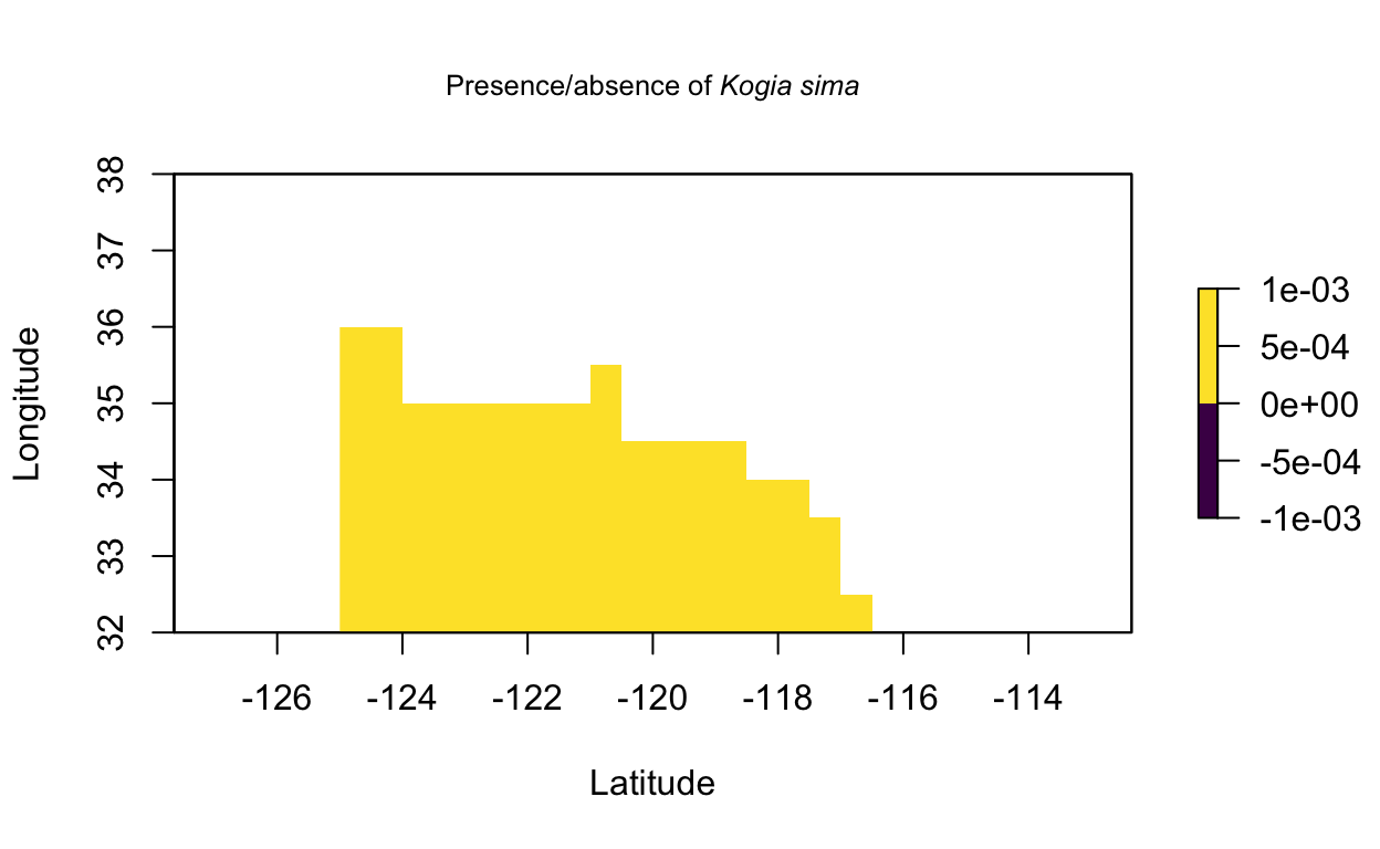
And for Kogia sima

Show code

plot(cet_presence$Kogia_sima, col = hcl.colors(n = 2))
title(expression(paste("Presence/absence of ", italic("Kogia sima"))), cex.main = 0.8,
      xlab = "Latitude", ylab = "Longitude")

Show code

# all look reasonable given the raw maps above

All of which look reasonable given the raw maps above. Nice!

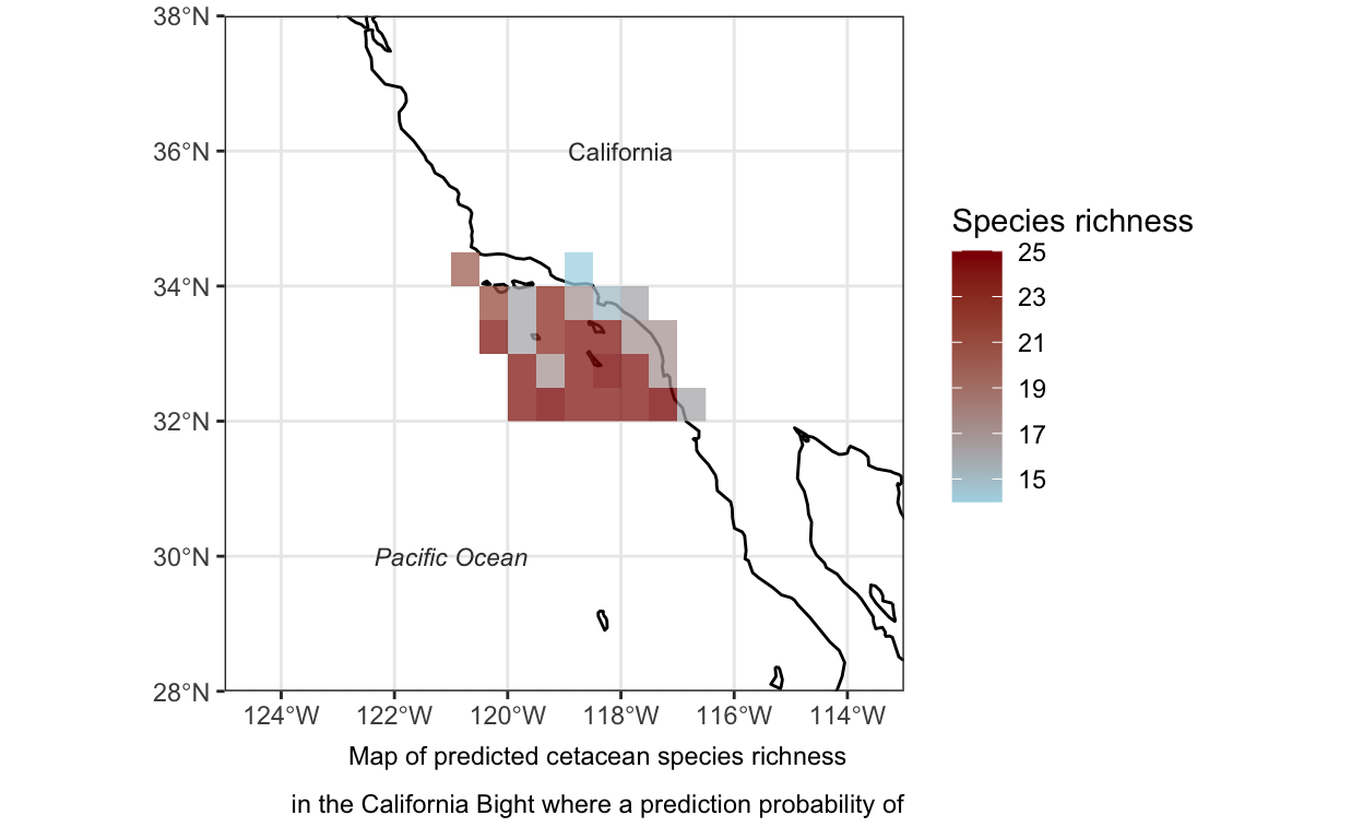
Calculate and plot potential species richness

Here we sum the “presence” of each organism in each cell and plot those results as an approximation of species richness.

Show code

cet_sum <- calc(cet_presence, sum, na.rm = FALSE) # get the sum of 1's (presence as we defined it) for the number of potential species in a grid cell

# can see what the summary looks like
# plot(cet_sum, col = hcl.colors(n = 20))

# get it into data.frame format for ggplot
cet_df <- raster::rasterToPoints(cet_sum) %>% # this is WGS84
  as.data.frame()

# get coastline data for reference
coasts <- ne_coastline(scale = "medium", returnclass = "sf")

# can visualize what the map looks like before using by running this code:
# plot(coasts) # this is WGS84

# plot with ggplot()
ggplot(data = coasts) +
  geom_sf() +
  coord_sf(xlim = c(-125, -113), ylim = c(28, 38), expand = FALSE) +
  annotate(geom = "text", x = -121, y = 30, label = "Pacific Ocean", 
     fontface = "italic", color = "grey22", size = 3) +
  annotate(geom = "text", x = -118, y = 36, label = "California", 
           color = "grey22", size = 3) +
  geom_raster(data = cet_df, aes(x = x, y = y, fill = layer), alpha = 0.75) +
  scale_fill_gradient(low = "lightblue", high = "darkred",
                           breaks=seq(from = 1, to = 25, by = 2)) +
  theme_bw() +
  theme(axis.title.x = element_blank(), 
     axis.title.y = element_blank(), 
     panel.border = element_rect(fill = NA)) +
  labs(fill = "Species richness",
       caption = expression(atop("Map of predicted cetacean species richness", "in the California Bight where a prediction probability of", "0.75 was considered a presence and below that was an absence")))