In this script I compare the words used in the most recent peer-reviewed paper by my PhD and Master’s adviser, where they were the senior (i.e. last) author. Although the lexicons and tools here are primarily for non-academic texts, this is a fun exercise to demonstrate what we can do with words in R. To see the code I used in each section click on the Show code option.
PhD adviser: Deron Burkepile
Read in my PhD adviser’s latest relevant publication, which was led by Dr. Leïla Ezzat.
Citation: - Ezzat, L., Lamy, T., Maher, R.L., Munsterman, K.S., Landfield, K.M., Schmeltzer, E.R., Clements, C.S., Thurber, R.L.V. and Burkepile, D.E., 2020. Parrotfish predation drives distinct microbial communities in reef-building corals. Animal Microbiome, 2(1), p.5.
Prepare the data
First, split the text up by line and trim excess white space
Show code
ezzat_tidy <- data.frame(ezzat_text) %>% # now each row is a different page
  mutate(text_full = str_split(ezzat_text, pattern = "\\n")) %>% # first slash just says look for \n as a string
# break it up using string split breaking wherever there is a line break
# now each line is an element -- then want each element
  unnest(text_full) %>% # now see repeated information but each line has it's own line
  mutate(text_full = str_trim(text_full)) %>% # get rid of excess white spaces
  slice(-1:-11) %>% # get rid of front matter/authors
  slice(-25:-37) %>% # remove license etc.
  slice(-545:-n()) %>% # remove supplement and citations
  slice(-1:-24) # also post-facto decide to remove abstract/just focus on main text
Then break up the PDF into logical sections for analysis
Show code
# break up the manuscript by traditional sections
ezzat_df <- ezzat_tidy %>%
  mutate(section = ifelse(str_detect(text_full, pattern = "Background"), "Introduction",
                  ifelse(str_detect(text_full, pattern = "Results"), "Results",
                  ifelse(str_detect(text_full, pattern = "Conclusion"), "Conclusion",
                  ifelse(str_detect(text_full, pattern = "Material and methods"), "Methods",

                          NA_character_))))) %>%
  fill(section) # fills in the NAs with the value above
  # need to know this is in order to use fill()
Remove numbers, citations, and figure/table references. Then get the data into tokenized text format, where one token is one single word using tidytext.
Show code
ezzat_tokens <- ezzat_df %>%
  mutate(text_full = gsub(x = text_full, pattern = "[0-9]+|[[:punct:]]|\\(.*\\)", replacement = "")) %>% # first get rid of numbers and citations because we are only analyzing the text
  # then remove Fig and Table labels
  mutate(text_full = gsub(x = text_full, pattern = "Fig.", replacement = "")) %>%
  mutate(text_full = gsub(x = text_full, pattern = "Tables", replacement = "")) %>%
  mutate(text_full = gsub(x = text_full, pattern = "Table", replacement = "")) %>%
  mutate(text_full = gsub(x = text_full, pattern = "Figure", replacement = "")) %>%
  mutate(text_full = gsub(x = text_full, pattern = "Figures", replacement = "")) %>%

  unnest_tokens(word, text_full) %>% # from tidytext
  select(-ezzat_text) # get rid of first column that holds no new information
Now remove stop words (i.e. common words like “the”, “is”, and “it”)
Show code
ezzat_nonstop_words <- ezzat_tokens %>%
  anti_join(stop_words) # knows to un-join by matching column name
# use ?stop_words to look at different stop_words lexicons


# count them by section (this is equivalent to group_by + summarize)
nonstop_counts <- ezzat_nonstop_words %>%
  count(section, word)

# find the top 10 words by section
top_10_words <- nonstop_counts %>%
  group_by(section) %>%
  arrange(-n) %>%
  slice(1:10) # keep top ten

top_10_words
# A tibble: 40 x 3
# Groups: section [4]
section word n
<chr> <chr> <int>
1 Conclusion coral 11
2 Conclusion corals 9
3 Conclusion parrotfish 8
4 Conclusion fish 4
5 Conclusion lobata 4
6 Conclusion microbiomes 4
7 Conclusion collected 3
8 Conclusion colonies 3
9 Conclusion colony 3
10 Conclusion corallivory 3
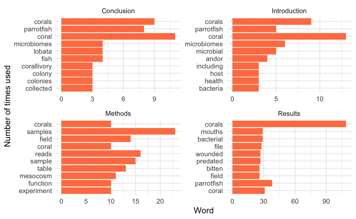
# … with 30 more rowsVisualize results
Visualize the top words
Show code
ggplot(data = top_10_words, aes(x = reorder(word, n), y = n)) +
  geom_col(fill = "coral") +
  facet_wrap(~section, scales = "free") + # need scales = "free" to make it so axes (incl. x axis) is not the same in each plot
  coord_flip() +
  ylab("Word") +
  xlab("Number of times used") +
  theme_minimal()
Make word clouds of the top 50 words in each section
Show code
intro_top50 <-
  nonstop_counts %>%
  filter(section == "Introduction") %>%
  arrange(-n) %>%
  slice(1:50)

intro_cloud_Der <- ggplot(data = intro_top50, aes(label = word)) +
  geom_text_wordcloud(aes(color = n, size = n)) +
  scale_size_area(max_size = 5.5) +
  ggtitle('Burkepile') +
  theme_void()

# see some words got cut off, but we'll leave those be for now
Show code
# can make one for methods
methods_top50 <-
  nonstop_counts %>%
  filter(section == "Methods") %>%
  arrange(-n) %>%
  slice(1:50)

meth_cloud_Der <- ggplot(data = methods_top50, aes(label = word)) +
  geom_text_wordcloud(aes(color = n, size = n)) +
  scale_colour_continuous(type = "viridis") +
  scale_size_area(max_size = 5.5) +
  theme_void() +
  ggtitle('Burkepile')


# or one for results
results_top50 <-
  nonstop_counts %>%
  filter(section == "Results") %>%
  arrange(-n) %>%
  slice(1:50)

res_cloud_Der <- ggplot(data = results_top50, aes(label = word)) +
  geom_text_wordcloud(aes(color = n, size = n)) +
  scale_colour_continuous(type = "gradient", low = "grey", high = "coral") +
  scale_size_area(max_size = 5.5) +
  theme_void() +
  ggtitle('Burkepile')


# or for the conclusion
concl_top50 <-
  nonstop_counts %>%
  filter(section == "Conclusion") %>%
  arrange(-n) %>%
  slice(1:50)

concl_cloud_Der <- ggplot(data = concl_top50, aes(label = word)) +
  geom_text_wordcloud(aes(color = n, size = n)) +
  scale_colour_continuous(type = "gradient", low = "orange", high = "darkorchid") +
  scale_size_area(max_size = 5.5) +
  theme_void() +
  ggtitle('Burkepile')
Conduct a sentiment analysis
Although this is not as relevant for academic papers like Ezzat et al., I’ll conduct a sentiment analysis for fun where we look at whether the words used have positive or negative connotations. This will be biased given that Ezzat et al. is talking about predation/wounding (and given that the lexicons are not meant for this kind of writing), but is a fun exercise.
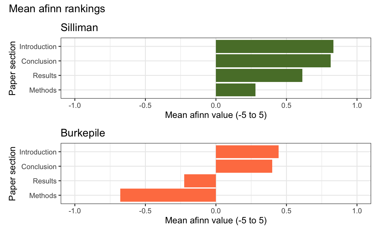
I’ll use the afinn lexicon that ranks words on a scale of -5 (very negative) to 5 (very positive). We’ll only keep words that have a counterpart in the afinn lexicon, which will dramatically change the words we analyze (again, this is better for other forms of text, but I thought it would be interesting anyways).
Show code
afinn_lex <- get_sentiments("afinn")

# join matching words
ezzat_afinn <- ezzat_nonstop_words %>%
  inner_join(get_sentiments("afinn"))

# can get total counts
afinn_counts <- ezzat_afinn %>%
  count(section, value) # see how positive and negative the values are for each section

# or could get mean value
afinn_means <- ezzat_afinn %>%
  group_by(section) %>%
  summarize(mean_afinn = mean(value))
Visualize results
Show code
afinn_Der <- ggplot(data = afinn_means, aes(x = reorder(section, mean_afinn), y = mean_afinn)) +
  geom_col(fill = "coral") +
  ylab("Mean afinn value (-5 to 5)") +
  xlab("Paper section") +
  coord_flip() +
  scale_y_continuous(limits = c(-1,1)) +
  theme_bw() +
  geom_vline(aes(xintercept = 0)) +
  ggtitle("Burkepile")
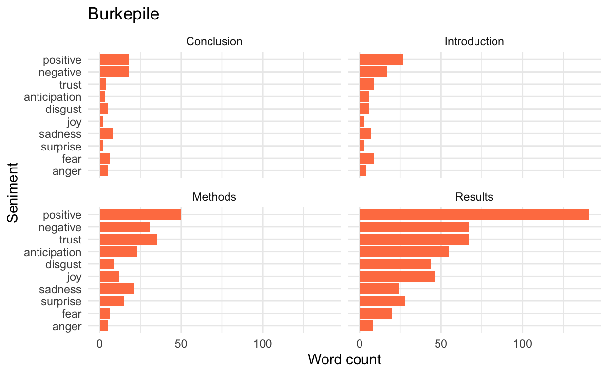
Or we could use a different lexicon, like the NRC lexicon.
Show code
ezzat_nrc <- ezzat_nonstop_words %>%
  inner_join(get_sentiments("nrc")) # have repeated values when there are multiple sentiments for a word

ezzat_nrc_counts <- ezzat_nrc %>%
  count(section, sentiment) # 10 sentiments total in nrc

nrc_Der <- ezzat_nrc_counts %>%
  ggplot(aes(x = reorder(sentiment, n), y = n)) +
  geom_col(fill = "coral") +
  facet_wrap(~section) +
  coord_flip() +
  xlab("Seniment") +
  ylab("Word count") +
  theme_minimal() +
  ggtitle("Burkepile") # these are only words that have a value in the nrc lexicon
M.S. adviser: Brian Silliman
Read in my M.S. adviser’s latest relevant publication, which was led by Dr. Qiang He.
Citation: - He, Q., Li, H., Xu, C., Sun, Q., Bertness, M.D., Fang, C., Li, B. and Silliman, B.R., 2020. Consumer regulation of the carbon cycle in coastal wetland ecosystems. Philosophical Transactions of the Royal Society B, 375(1814), p.20190451.
Prepare the data
First, split the text up by line and trim excess white space
Show code
he_tidy <- data.frame(he_text) %>%
  mutate(text_full = str_split(he_text, pattern = "\\n")) %>%
  unnest(text_full) %>%
  mutate(text_full = str_trim(text_full)) %>% # get rid of excess white spaces
  slice(-1:-43) %>% # get rid of front matter/authors/abstract
  slice(-500:-n()) # remove citations, etc.
Then break up the PDF into logical sections for analysis
Show code
# break up the manuscript by traditional sections
# these are slightly different than Ezzat et al, but we'll keep the names consistent
he_df <- he_tidy %>%
  mutate(section = ifelse(str_detect(text_full, pattern = "1. Introduction"), "Introduction",
                  ifelse(str_detect(text_full, pattern = "2. Materials and methods"), "Methods",
                  ifelse(str_detect(text_full, pattern = "3. Results"), "Results",
                  ifelse(str_detect(text_full, pattern = "4. Discussion"), "Conclusion",

                          NA_character_))))) %>%
  fill(section)
Remove numbers, citations, and figure/table references. Then get the data into tokenized text format, where one token is one single word using tidytext.
Show code
he_tokens <- he_df %>%
  mutate(text_full = gsub(x = text_full, pattern = "[0-9]+|[[:punct:]]|\\(.*\\)", replacement = "")) %>% # first get rid of numbers and citations because we are only analyzing the text
  # then remove Fig and Table labels and other artifacts
  mutate(text_full = gsub(x = text_full, pattern = "figure", replacement = "")) %>%
  mutate(text_full = gsub(x = text_full, pattern = "figures", replacement = "")) %>%
  mutate(text_full = gsub(x = text_full, pattern = "table", replacement = "")) %>%
  mutate(text_full = gsub(x = text_full, pattern = "tables", replacement = "")) %>%
  mutate(text_full = gsub(x = text_full, pattern = "Phil. Trans. R. Soc. B", replacement = "")) %>%
  mutate(text_full = gsub(x = text_full, pattern = "royalsocietypublishing.org/journal/rstb", replacement = "")) %>%
  mutate(text_full = gsub(x = text_full, pattern = "royalsocietypublishingorgjournalrstb", replacement = "")) %>%

  unnest_tokens(word, text_full) %>% # from tidytext
  select(-he_text) # get rid of first column that holds no new information
Now remove stop words (i.e. common words like “the”, “is”, and “it”)
Show code
he_nonstop_words <- he_tokens %>%
  anti_join(stop_words)


# count them by section (this is equivalent to group_by + summarize)
nonstop_counts <- he_nonstop_words %>%
  count(section, word)

# find the top 10 words by section
top_10_words <- nonstop_counts %>%
  group_by(section) %>%
  arrange(-n) %>%
  slice(1:10) # keep top ten

top_10_words
# A tibble: 40 x 3
# Groups: section [4]
section word n
<chr> <chr> <int>
1 Conclusion carbon 40
2 Conclusion herbivores 26
3 Conclusion effects 21
4 Conclusion coastal 20
5 Conclusion cycle 18
6 Conclusion processes 15
7 Conclusion wetlands 15
8 Conclusion consumers 14
9 Conclusion soil 13
10 Conclusion herbivore 12
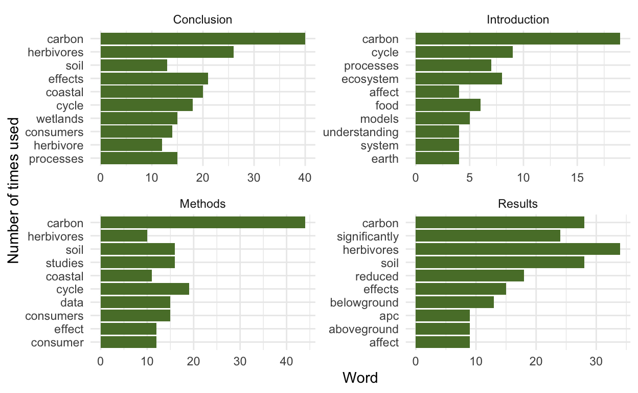
# … with 30 more rowsVisualize results
Visualize the top words
Show code
ggplot(data = top_10_words, aes(x = reorder(word, n), y = n)) +
  geom_col(fill = "#597D35") +
  facet_wrap(~section, scales = "free") + # need scales = "free" to make it so axes (incl. x axis) is not the same in each plot
  coord_flip() +
  ylab("Word") +
  xlab("Number of times used") +
  theme_minimal()
Make word clouds of the top 50 words in each section
Show code
intro_top50 <-
  nonstop_counts %>%
  filter(section == "Introduction") %>%
  arrange(-n) %>%
  slice(1:50)

intro_cloud_Sill <- ggplot(data = intro_top50, aes(label = word)) +
  geom_text_wordcloud(aes(color = n, size = n)) +
  scale_size_area(max_size = 5.5) +
  ggtitle('Silliman') +
  theme_void()
# see some words got cut off, but we'll leave those be for now
Show code
# can make one for methods
methods_top50 <-
  nonstop_counts %>%
  filter(section == "Methods") %>%
  arrange(-n) %>%
  slice(1:50)

meth_cloud_Sill <- methods_cloud <- ggplot(data = methods_top50, aes(label = word)) +
  geom_text_wordcloud(aes(color = n, size = n)) +
  scale_colour_continuous(type = "viridis") +
  scale_size_area(max_size = 5.5) +
  ggtitle('Silliman') +
  theme_void()


# or one for results
results_top50 <-
  nonstop_counts %>%
  filter(section == "Results") %>%
  arrange(-n) %>%
  slice(1:50)

res_cloud_Sill <- ggplot(data = results_top50, aes(label = word)) +
  geom_text_wordcloud(aes(color = n, size = n)) +
  scale_colour_continuous(type = "gradient", low = "grey", high = "coral") +
  scale_size_area(max_size = 5.5) +
  ggtitle('Silliman') +
  theme_void()


# or for the conclusion
concl_top50 <-
  nonstop_counts %>%
  filter(section == "Conclusion") %>%
  arrange(-n) %>%
  slice(1:50)

concl_cloud_Sill <- ggplot(data = concl_top50, aes(label = word)) +
  geom_text_wordcloud(aes(color = n, size = n)) +
  scale_colour_continuous(type = "gradient", low = "orange", high = "darkorchid") +
  scale_size_area(max_size = 5.5) +
  ggtitle('Silliman')  +
  theme_void()
Plot them together to compare:
Show code
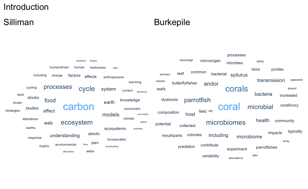
(intro_cloud_Sill + intro_cloud_Der) + plot_annotation(
  title = 'Introduction')
Show code
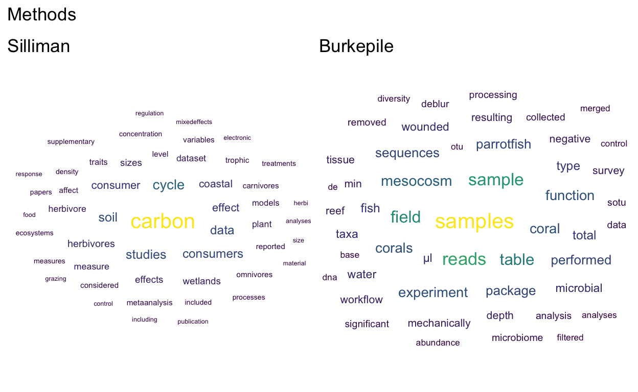
(meth_cloud_Sill + meth_cloud_Der) + plot_annotation(
  title = 'Methods')
Show code
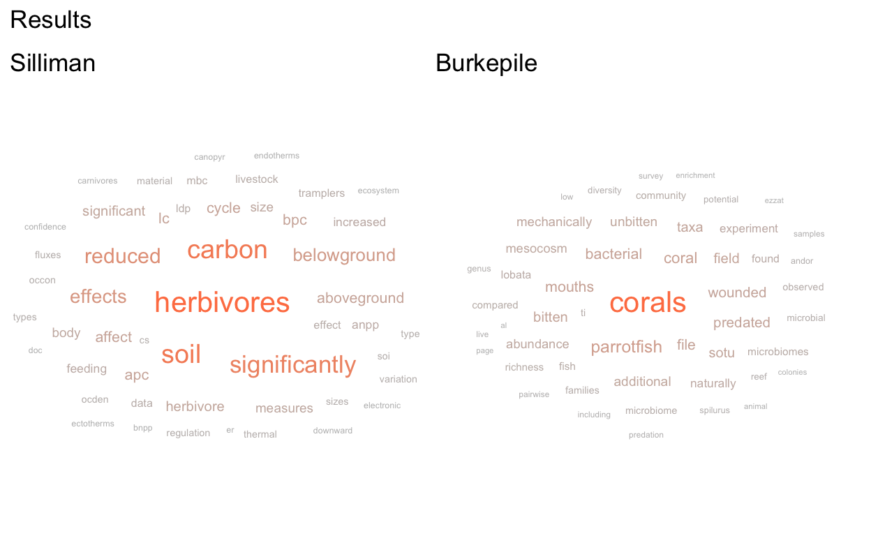
(res_cloud_Sill + res_cloud_Der) + plot_annotation(
  title = 'Results')
Show code
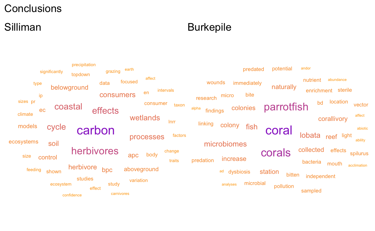
(concl_cloud_Sill + concl_cloud_Der) + plot_annotation(
  title = 'Conclusions')
Conduct a sentiment analysis
Start with the afinn lexicon again that ranges from -5 to 5.
Show code
afinn_lex <- get_sentiments("afinn")

# join matching words
he_afinn <- he_nonstop_words %>%
  inner_join(get_sentiments("afinn"))

# can get total counts
afinn_counts <- he_afinn %>%
  count(section, value) # see how positive and negative the values are for each section

# or could get mean value
afinn_means <- he_afinn %>%
  group_by(section) %>%
  summarize(mean_afinn = mean(value))
Visualize results
Show code
afinn_Sill <- ggplot(data = afinn_means, aes(x = reorder(section, mean_afinn), y = as.numeric(mean_afinn))) +
  geom_col(fill = "#597D35") +
  ylab("Mean afinn value (-5 to 5)") +
  xlab("Paper section") +
  coord_flip() +
  scale_y_continuous(limits = c(-1,1)) +
  theme_bw() +
  geom_vline(aes(xintercept = 0)) +
  ggtitle("Silliman")
Plot them together for comparison
Show code
afinn_Sill / afinn_Der + plot_annotation(
  title = "Mean afinn rankings")
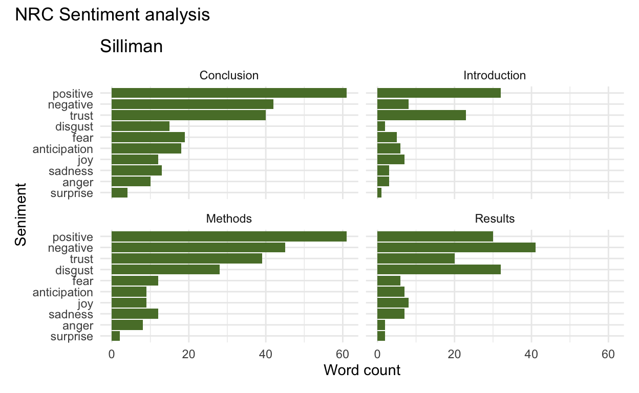
Then we use the NRC lexicon again.
Show code
he_nrc <- he_nonstop_words %>%
  inner_join(get_sentiments("nrc")) # have repeated values when there are multiple sentiments for a word

he_nrc_counts <- he_nrc %>%
  count(section, sentiment) # 10 sentiments total in nrc

nrc_Sill <- he_nrc_counts %>%
  ggplot(aes(x = reorder(sentiment, n), y = n)) +
  geom_col(fill = "#597D35") +
  facet_wrap(~section) +
  coord_flip() +
  xlab("Seniment") +
  ylab("Word count") +
  theme_minimal() +
  ggtitle("Silliman")
Plot them together