Interactive & choropleth mapping

In this post I use publically-available data on California Oil Spills to show how to quickly and easily create an interactive map using tmap. I also use these data to create a choropleth map showing the number of inland oil spills per county.

Load the data

These data are on oil spills in California. They were downloaded as a shapefile from the California Department of Fish and Wildlife (read more about the dataset here: https://map.dfg.ca.gov/metadata/ds0394.html)

Show code

oil_spills <- read_sf(here("_posts", "2021-02-24-interactivemap", "data", "ds394", "ds394.shp"))

oil_spills %>% st_crs # NAD 1983

Coordinate Reference System:
  User input: NAD83 / California Albers 
  wkt:
PROJCRS["NAD83 / California Albers",
    BASEGEOGCRS["NAD83",
        DATUM["North American Datum 1983",
            ELLIPSOID["GRS 1980",6378137,298.257222101,
                LENGTHUNIT["metre",1]]],
        PRIMEM["Greenwich",0,
            ANGLEUNIT["degree",0.0174532925199433]],
        ID["EPSG",4269]],
    CONVERSION["California Albers",
        METHOD["Albers Equal Area",
            ID["EPSG",9822]],
        PARAMETER["Latitude of false origin",0,
            ANGLEUNIT["degree",0.0174532925199433],
            ID["EPSG",8821]],
        PARAMETER["Longitude of false origin",-120,
            ANGLEUNIT["degree",0.0174532925199433],
            ID["EPSG",8822]],
        PARAMETER["Latitude of 1st standard parallel",34,
            ANGLEUNIT["degree",0.0174532925199433],
            ID["EPSG",8823]],
        PARAMETER["Latitude of 2nd standard parallel",40.5,
            ANGLEUNIT["degree",0.0174532925199433],
            ID["EPSG",8824]],
        PARAMETER["Easting at false origin",0,
            LENGTHUNIT["metre",1],
            ID["EPSG",8826]],
        PARAMETER["Northing at false origin",-4000000,
            LENGTHUNIT["metre",1],
            ID["EPSG",8827]]],
    CS[Cartesian,2],
        AXIS["easting (X)",east,
            ORDER[1],
            LENGTHUNIT["metre",1]],
        AXIS["northing (Y)",north,
            ORDER[2],
            LENGTHUNIT["metre",1]],
    USAGE[
        SCOPE["unknown"],
        AREA["USA - California"],
        BBOX[32.53,-124.45,42.01,-114.12]],
    ID["EPSG",3310]]

Read in county borders

Show code

ca_counties <- read_sf(here("_posts", "2021-02-24-interactivemap", "data", "ca_counties", "CA_Counties_TIGER2016.shp")) %>% 
  select(NAME, ALAND) %>% 
  rename(county_name = NAME, land_area = ALAND) %>% 
  st_transform(crs = st_crs(oil_spills)) # want crs to match oil spill data

# double check CRS
st_crs(oil_spills) == st_crs(ca_counties) # looks good

[1] TRUE

Show code

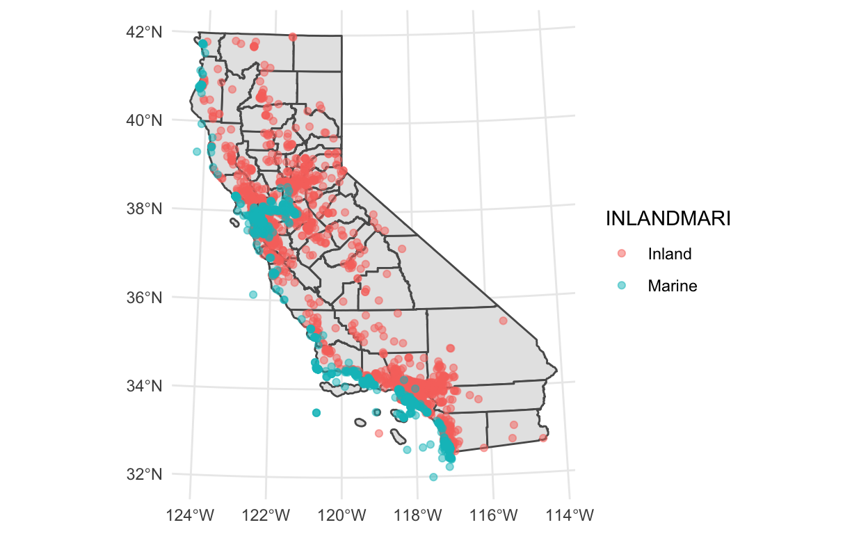
ggplot() +
  geom_sf(data = ca_counties) +
  geom_sf(data = oil_spills, aes(color = INLANDMARI), alpha = 0.5) +
  theme_minimal()

Make an interactive map

Now make it interactive

Show code

# set viewing mode to interactive
tmap_mode(mode = "view")

# make map with the polygon fill color updated by variable 'land_area', updating the color palette to "BuGn"), then add another shape layer for the sesbania records (added as dots)
tm_shape(ca_counties) +
  tm_polygons(col = "white") +
  tm_shape(oil_spills) +
  tm_dots(col = "INLANDMARI", title = "Area") +
  tm_basemap("Esri.WorldTopoMap") # this sets the basemap--I changed it to the topographic map for fun but there are 3 options and one can change it in the GUI

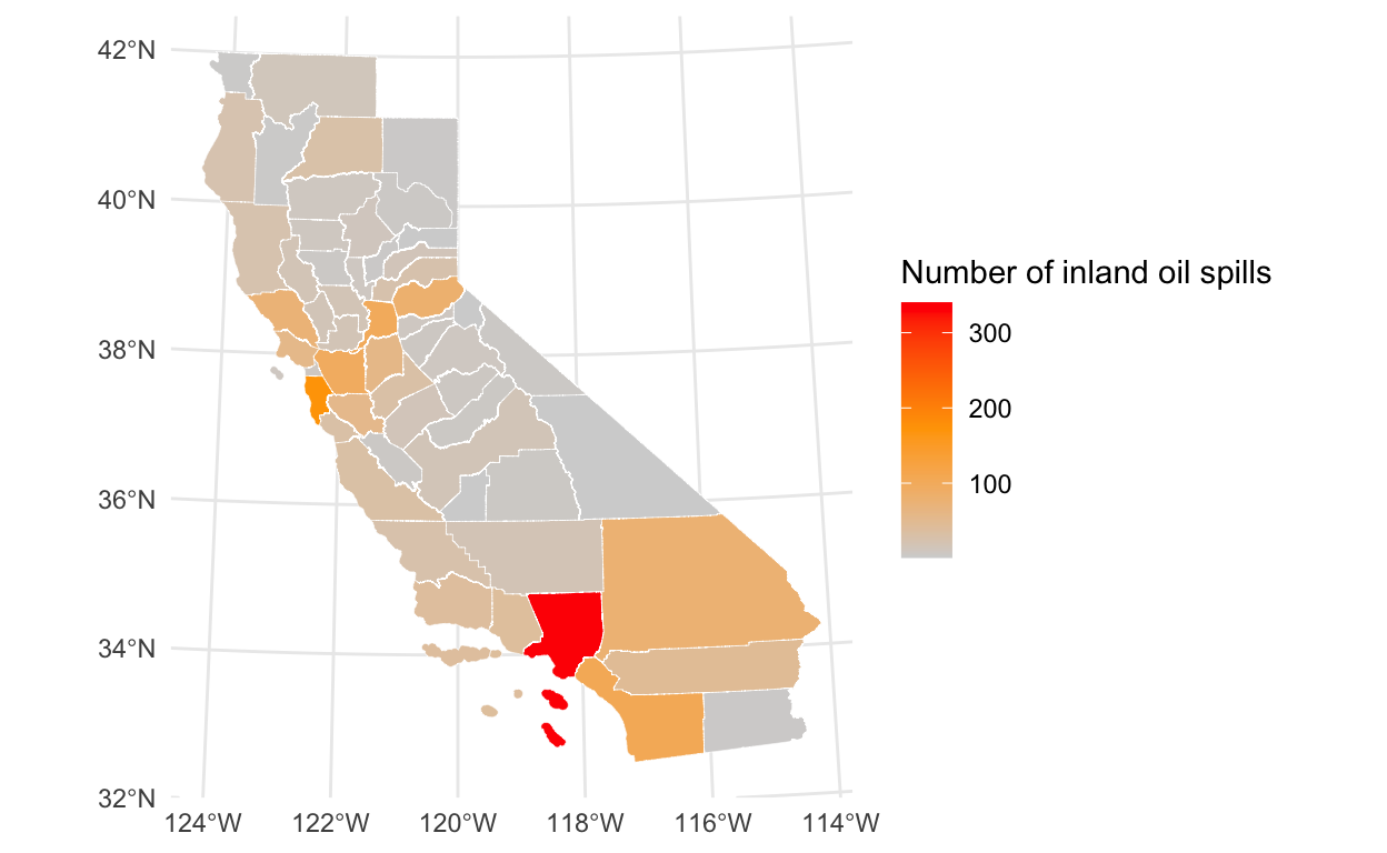
Create the choropleth map

Now make a choropleth map where the fill color for each county depends on the count of inland oil spill events for 2008

Show code

# join data points to counties
oil_counties <- ca_counties %>% 
  st_join(oil_spills)

oil_count <- oil_counties %>% 
  filter(INLANDMARI == "Inland") %>% 
  count(LOCALECOUN) 


# plot
ggplot(data = oil_count) +
  geom_sf(aes(fill = n), color = "white", size = 0.1) + 
  scale_fill_gradientn(colors = c("lightgray", "orange", "red")) +
  theme_minimal() +
  labs(fill = "Number of inland oil spills")